One of the most straightforward tasks in machine learning is approximating a given mathematical function. Mainly because it’s very easy to know and measure what’s right and what’s wrong: for any given point we can simply calculate the correct answer. Thus the dataset is very easy to obtain.

In Statistics and Machine Learning, this task is called “regression” (as opposed to “classification") because we’re trying to estimate an underlying distribution (or a particular point of this distribution) instead a classifying a given point.

In this post I’m going to describe how to set up a Multilayer Perceptron for regression on any arbitrary mathematical function.

#  Function y

We’ll start with this combined sinusoid:

y(x) = sin(2π * x) + sin(5π * x) with x = -1:0.002:1

First, we implement the above function in Python:

1
2
3
4

import numpy as np

def y(x):
    return (np.sin(2*np.pi*x) + np.sin(5*np.pi*x))

Which we then use to generate our dataset:

1
2

x_vals = np.arange(-1,1,0.002)
y_vals = y(x_vals)

Depending on which activation function we use for our neurons, we also need to normalize the data between -1 and 1 (e.g. for sigmoid). We store the y_max value so we can restore the original values later (e.g. for plotting).

1
2

y_max = y_vals.max()
y_vals /= y_max

Then we split our dataset into a training and a testing set. Typical splits range anywhere between 70/30 and 90/10, so we’re using a 80/20 split here:

1
2
3

from sklearn.model_selection import train_test_split

x_train, x_test, y_train, y_test = train_test_split(x_vals, y_vals, test_size=0.20)

We could also manually do this, but Scikit-learn already provides a nice function that splits and shuffles the dataset.

Let’s have a look at what our data currently looks like:

1
2
3
4
5
6

import matplotlib.pyplot as plt

plt.figure()
plt.plot(x_train, y_train, 'o')
plt.plot(x_test, y_test, 'x')
plt.show()

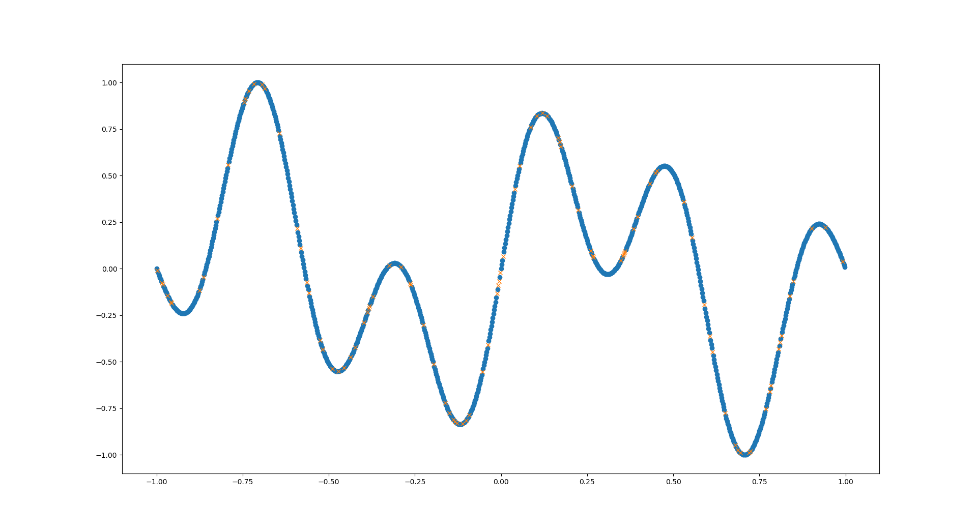
The blue dots are the training data for our network, the yellow crosses are the test data - the network should predict these later!

Since we have 1D input data for our network, we need to reshape it:

1
2

x_train = x_train.reshape(-1,1)
x_test = x_test.reshape(-1,1)

After all this setup, we can move on to the heart of our application. We use the MLPRegressor function from Scikit-learn to set up our MLP. I cannot explain all its parameters here, so go have a look at its documentation. In the example below we are using just a single hidden layer with 30 neurons.

 1
 2
 3
 4
 5
 6
 7
 8
 9
10

from sklearn.neural_network import MLPRegressor

mlp = MLPRegressor(
    hidden_layer_sizes=[30],
    max_iter=1000,
)

mlp.fit(x_train,y_train)

predictions = mlp.predict(x_test)

Great, we have our predictions! But what to do with them? First we can visualize them, of course:

1
2

plt.plot(x_test, predictions, 'ro')
plt.show()

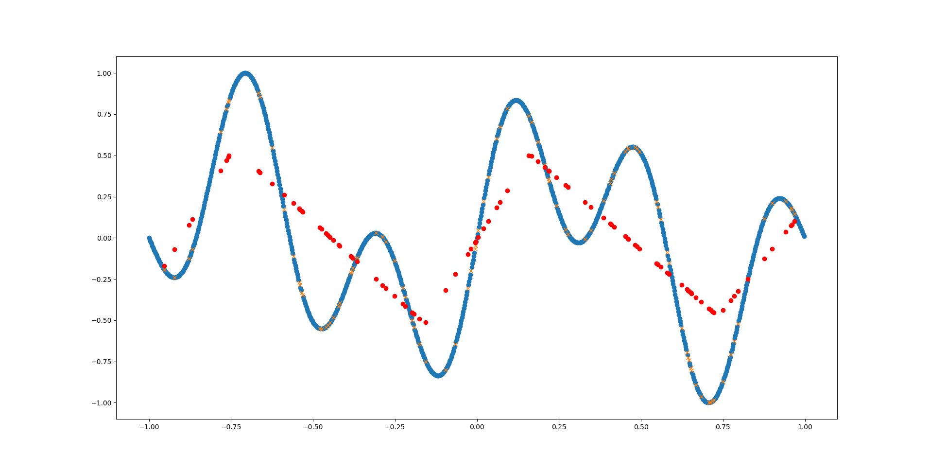
In the above example we can see that the network has barely detected the first (main) sinus function. The network simply does not have enough inherent complexity to model the already complex sinus function - let alone two of them together!

But we can also look at the predictions in a more abstract way, by calculating the mean squared error (MSE):

1
2
3

from sklearn.metrics import mean_squared_error

mse = mean_squared_error(y_test, predictions)

Essentially this will just go over all predictions, calculate their distance from the correct answer, square it and sum them all up.

Since the prediction performance is really terrible and our network is really tiny, we can try adding a few more layers and neurons:

1
2
3
4

mlp = MLPRegressor(
    hidden_layer_sizes=[10,30,10],
    max_iter=1000,
)

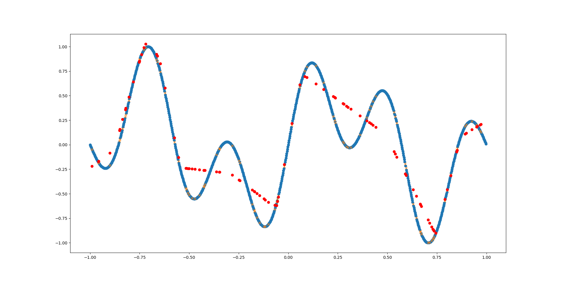
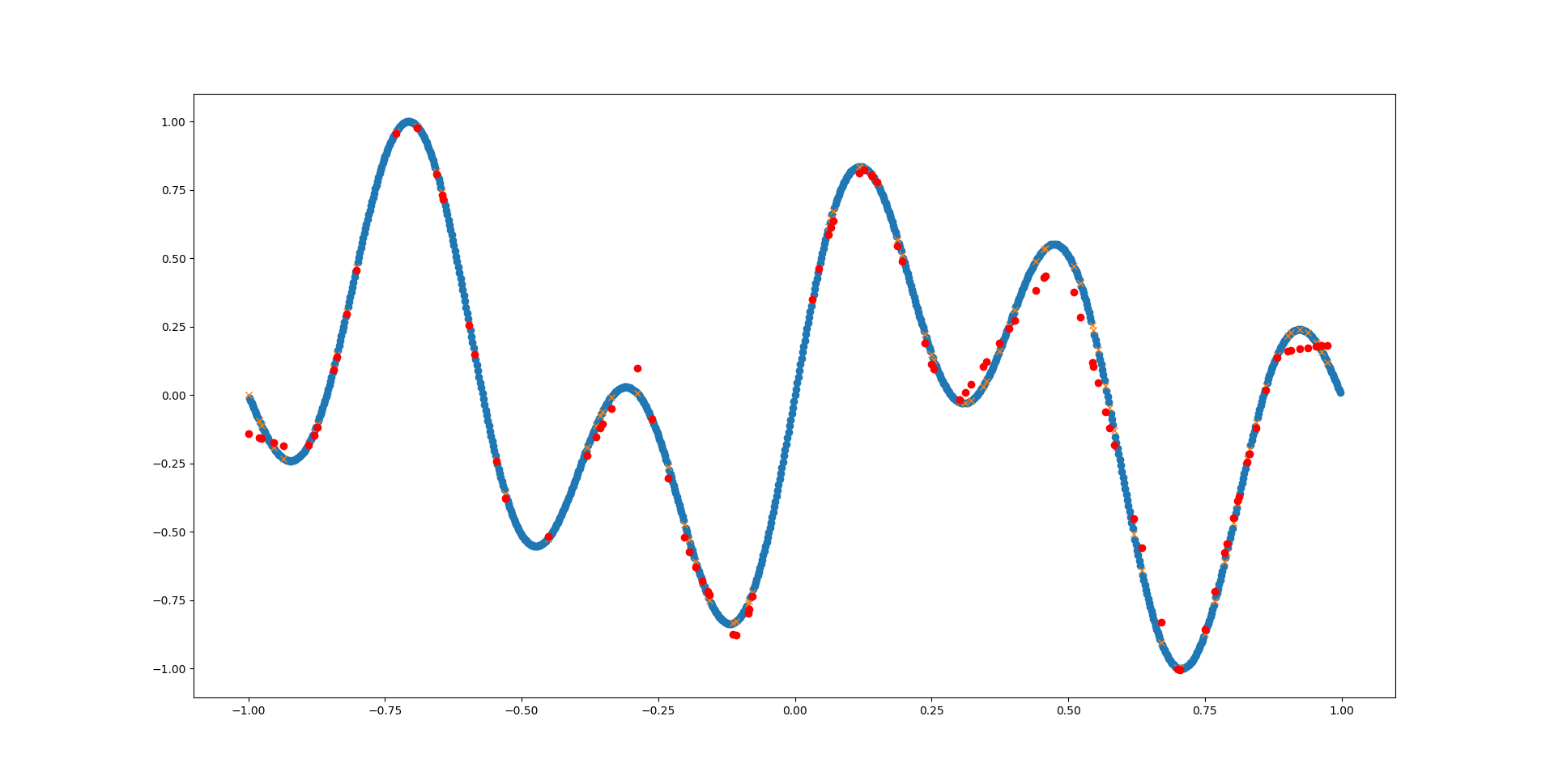
That looks much better already! Go ahead and play around with MLPRegressor’s parameters and see how well you can fit the function.

#  Function z

The same can be done for a two-dimensional function like the following:

z(x,y) = exp( -(x² + y²) / 0.1)

We begin again by implementing our function in Python:

1
2

def z(x,y):
    return np.exp(-(np.square(x) + np.square(y))/0.1)

So far so good. To create the dataset this time, we need a list of (x,y) coordinates and calculate the corresponding z value:

1
2
3

x = np.arange(-1,1,0.05)
xy = [(j,k) for j in x for k in x]
out = [z(p[0],p[1]) for p in xy]

Depending on the function you might want to normalize the output values at this point. For the above function this is not required, since the value of the exponential function for negative inputs is between 0 and 1 anyway.

Again, split the dataset into training and testing data:

1

x_train, x_test, y_train, y_test = train_test_split(xy, out)

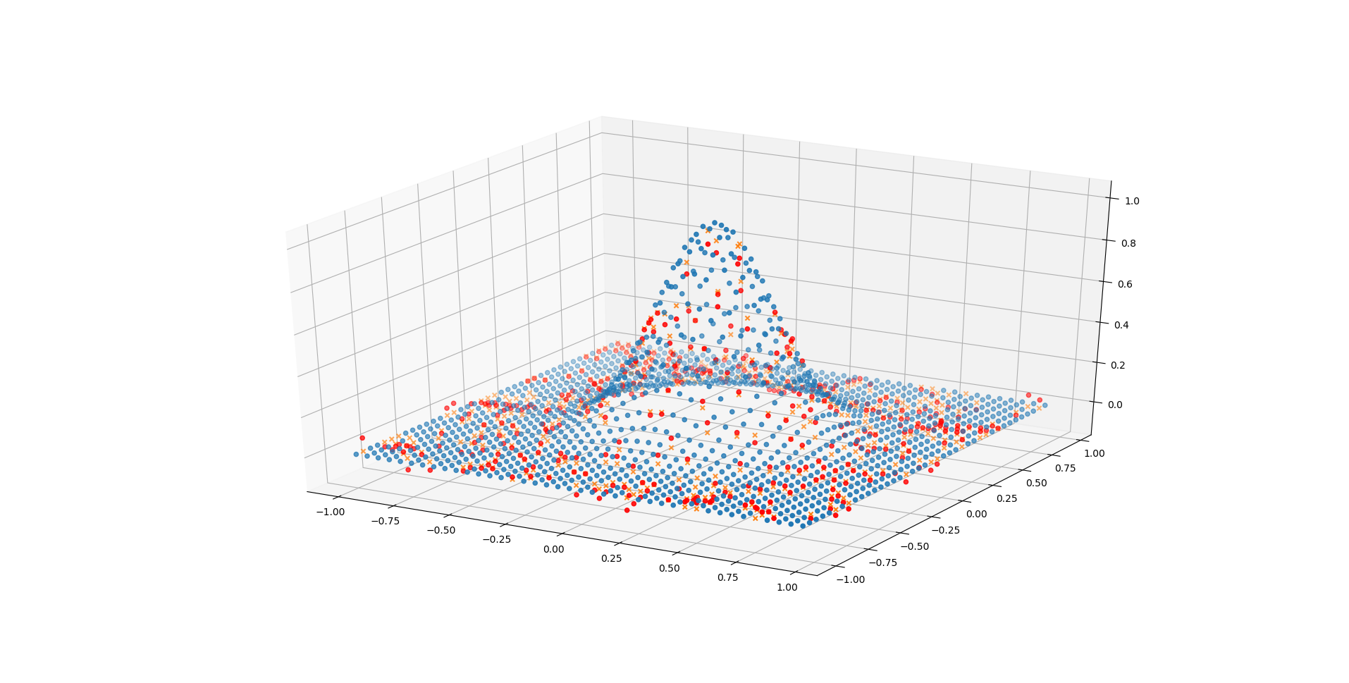
And depict it as a 3D plot:

 1
 2
 3
 4
 5
 6
 7
 8
 9
10
11
12
13
14
15
16
17
18
19

import matplotlib.pyplot as plt
from mpl_toolkits.mplot3d import Axes3D

fig = plt.figure()
ax = fig.gca(projection='3d')

# plot train data points
x1_vals = np.array([p[0] for p in x_train])
x2_vals = np.array([p[1] for p in x_train])

ax.scatter(x1_vals, x2_vals, y_train)

# plot test data points
x1_vals = np.array([p[0] for p in x_test])
x2_vals = np.array([p[1] for p in x_test])

ax.scatter(x1_vals, x2_vals, y_test, marker='x')

plt.show()

Here we need to do some data structure crafting to get the points in the right shape for plotting. First we split the list of (x,y) points into one array containing the indices of the x1 axis (called x1_vals) and another array containing the indices of the x2 axis (called x2_vals). Then we can use the indices along with the function output values to create a 3D scatter plot. Due to the equidistant spacing of the data points this nicely looks like a surface. The same is done for the test data.

The training and prediction part is the same as before:

 1
 2
 3
 4
 5
 6
 7
 8
 9
10
11
12
13
14

# set up network with parameters
mlp = MLPRegressor(
    hidden_layer_sizes=[20],
    max_iter=1000,
    tol=0,
)

# train network
mlp.fit(x_train,y_train)

# test
predictions = mlp.predict(x_test)

mse = mean_squared_error(y_test, predictions)

And plot the predictions again:

1
2
3

ax.scatter(x1_vals, x2_vals, predictions, c='red')

plt.show()

Even with only a single hidden layer containing 20 neurons the network performs quite well on this task (compared to the previous one). This because the underlying shape is much simpler (symmetric exponential function), therefore a less complex network is required to adequately fit it.

Go ahead and see how small you can make the network before loosing too much fidelity!

#  References

• Full Source Code func_y.py, func_z.py
• Numpy
• Scikit-learn
• Matplotlib pyplot
• Python 3